Estimating Upwelling from Surface Wind using Python

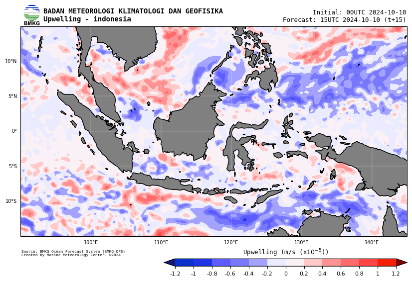
Upwelling region can be estimated from surface wind. This is done through Ekman Pumping Velocity, derivied from wind stress and wind stress curl. Following Simanjuntak and Lin (2022)¹, this article will explain step by step calculation on how to derivied Ekman Pumping Velocity to determine upwelling region based on multidimensional gridded data.

Data

We will use data from BMKG-OFS, produced by Center for Marine Meteorology. This data contains $u$ and $v$ component of wind vector. It has $0.0625° \times 0.0625°$ spatial resolution and 3-hourly temporal resolution.

You can request the sample of the data by contacting me, or feel free to use your own data, you only need $u$ and $v$ component of wind vector in gridded field.

Surface Wind Stress ($\tau$)

The sea surface wind data can be converted into wind stress ($\tau$) based on the following equation.

\[\tau = \rho_a C_d U^{2}_{10}\]

where $\rho_a$ is the air density, $C_d$ is drag coeficient, and $U^{2}_{10}$ is wind speed at a 10m height.

Wind Stress Curl

Wind stress curl is calculated from wind stress vector component.

\[curl = \frac{\partial\tau_y}{\partial x} - \frac{\partial \tau_x}{\partial y}\]

Ekman Pumping Velocity

\[EPV = - \frac{curl}{\rho_w f}\]

where $\rho_w$ is the water density and $f$ is the coriolis parameter.

Scripting with Python

import numpy as np 
import xarray as xr 
from scipy.ndimage import gaussian_filter
from datetime import datetime, timedelta

class Upwelling:
    def __init__(self):
        self.__RHOA__  = 1.225
        self.__RHOW__  = 1028
        self.__DC__    = 1.25e-3
        self.__OMEGA__ = 7.29e-5

    def calc_wind_stress(self, dset:xr.Dataset, uwnd:str, vwnd:str) -> xr.Dataset:
        dset['uwnd_stress'] = (self.__RHOA__*self.__DC__*dset[uwnd])*(np.sqrt(dset[uwnd]**2 + dset[vwnd]**2))
        dset['vwnd_stress'] = (self.__RHOA__*self.__DC__*dset[vwnd])*(np.sqrt(dset[uwnd]**2 + dset[vwnd]**2))
        return dset 

    def calc_wind_curl(self, dset:xr.Dataset, uwnd_stress:str, vwnd_stress:str, lat:str) -> xr.Dataset:
        dy = 0.0625*111320 # adjust to your latitude resolution
        dx = 0.0625*111320 # adjust to your longitude resolution

        corioli = 2 * self.__OMEGA__ * np.sin(np.deg2rad(dset[lat]))
        dset['corioli'] = corioli.expand_dims({'time': dset.dims['time'], 'lon': dset.dims['lon']}, axis=(0, 2)) # adjust to your data, in this case the order is time-lat-lon
        d_tau_y_dx = np.gradient(dset[vwnd_stress], dx, axis=2)
        d_tau_x_dy = np.gradient(dset[uwnd_stress], dy, axis=1)
        wind_curl = (d_tau_y_dx - d_tau_x_dy)
        dset['wind_curl'] = (('time', 'lat', 'lon'), wind_curl)
        return dset

    def calc_epv(self, dset:xr.Dataset, wind_curl:str, corioli:str) -> xr.Dataset:
        epv = dset[wind_curl] / (self.__RHOW__ * dset[corioli])
        dset['epv'] = epv
        return dset

Execution and Plotting

class uwPlotter(plotter): 
    '''
    You can make your own plotter, this class is inherit from the other class (plotter) which contains hundreds of lines to plot the data
    '''
    def __init__(self):
        super().__init__()
        self.__TIMENOW__ = datetime.now()

    def gaussian_blur(self, dset, sigma=3):
        dset['epv'] = xr.where(np.isfinite(dset['epv']), dset['epv'], 0)
        dset['epv'] = xr.where((dset['epv'] > -0.00001) & (dset['epv'] < 0.00001), dset['epv'], 0)
        dset['epv'] = dset['epv']*100000
        blurred_data = gaussian_filter(dset['epv'].values, sigma=sigma)
        dset['epv'] = xr.DataArray(blurred_data, coords=dset['epv'].coords, dims=dset['epv'].dims)
        return dset
    
    def run_plot_uwp(self, baserun, tsel, ds, area_name, out_dir):
        ds = ds.isel(time=tsel)
        forecast = pd.to_datetime(ds.time.data)
        logging.info(f"======Running Plotter for {area_name} | baserun: {baserun} | forecast: {forecast}======")
        ds = self.gaussian_blur(ds)
        self.run_plot(
            ds=ds,
            var='epv',
            wilpel='wilpel',
            wilpel_name=area_name,
            map_area=area_name,
            out_dir=out_dir,
            baserun=baserun,
            forecast=forecast,
        )

The script above is a part of the production script to generate upwelling maps that can be seen through this link https://maritim.bmkg.go.id/ofs-static, select Model: Ina-flow and Parameter: Upwelling.

Sample of Upwelling maps

References

1. Simanjuntak, F., & Lin, T. H. (2022). Monsoon effects on chlorophyll-a, sea surface temperature, and ekman dynamics variability along the southern coast of lesser Sunda islands and its relation to ENSO and IOD based on satellite observations. Remote Sensing, 14(7), 1682. https://doi.org/10.3390/rs14071682 ↩